4.4. Light-Duty VMT and New Vehicle Sales Forecasting#
4.4.1. Light-Duty VMT Forecast#
EMFAC2025’s forecasting methodology for future light-duty VMT generally follows the same process as EMFAC2021 and EMFAC2017. For calendar years following the base year (2022), VMT is forecasted under two regimes (near-term and long-term forecasts), summarized in Table 4.4.
Years |
VMT Forecasting Methodology |
|---|---|
2023 to 2027 |
Use socioeconomic variables to forecast trends in VMT per capita and then multiply by human population to calculate VMT |
2028 to 2050 |
VMT per capita is constant, and VMT trends follow the human population growth rate |
For near-term VMT forecasting (years 2023 to 2027), CARB staff apply a multivariate linear regression analysis using a range of socioeconomic variables to predict trends in VMT per capita. The socioeconomic variables that were considered as possible predictors of VMT per capita are listed in Table 4.5. The regression analysis is conducted at a statewide, annual scale for the historical period from 2003 to 2022. The year 2020 is excluded from the model fitting process, since it had an anomalous reduction in VMT per capita due to the COVID-19 pandemic. For purposes of this multivariate regression analysis, historical VMT was approximated based on gasoline sales data provided by the California Department of Tax and Fee Administration (CDTFA) and fuel efficiency estimates (miles per gallon) for light-duty vehicle classes from EMFAC2021.
VMT Predictor Variable |
Data Source |
|---|---|
California human population |
California Department of Finance (DOF, 2023) |
Gas prices |
California Energy Commission (CEC, 2023) |
Federal gross domestic product |
Congressional Budget Office (CBO, 2023) |
Federal interest rate |
|
Housing starts |
UCLA Anderson Economic Forecast (UCLA, 2023) |
Unemployment rate |
|
Disposable income |
CARB staff evaluated various combinations of these variables to identify the model that best captures historical trends in VMT per capita. A computer program was developed to automate the calculation of ordinary least squares regression fits for every possible combination of the above candidate variables. Initially, staff considered multivariate models with up to five predictor variables, including 1- and 2-year lagged versions of each variable to account for potential delayed effects. However, given the limited sample size (19 annual data points from calendar years 2003 to 2022), staff restricted the model to two predictor variables and excluded lagged terms. This decision aligns with general statistical guidance recommending a minimum of 10 observations per predictor variable to reduce the risk of overfitting. After generating all possible regression models, the following criteria were applied to identify the most appropriate model:
The \(p\)-values for each predictor variable must be less than 0.05
The adjusted \(R^2\) value must be greater than 0.85
The sign of the variable coefficients must make logical sense (e.g., the sign of the gas price coefficient should be negative, since higher gas prices should not lead to higher VMT).
After applying these criteria, the two-variable model with the highest adjusted \(R^2\) was selected (Figure 4.9). This model had an adjusted \(R^{2}\) value of 0.89. The \(p\)-values for each variable indicated statistical significance (Table 4.6). The chosen model that best predicted historical VMT per capita was:
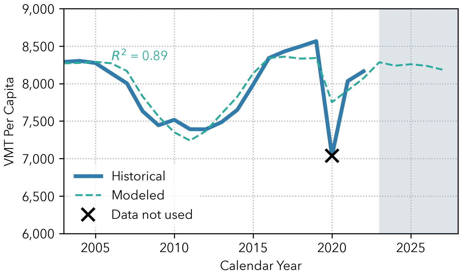
Figure 4.9: Vehicle Miles Traveled per Capita from 2003 to 2022: Historical vs. Modeled#
Variable |
\(p\)-value |
|---|---|
\(y\)-intercept |
\(1.76\times10^{-17}\) |
Unemployment rate (%) |
\(7.28\times10^{-8}\) |
Gas price (2021 USD) |
\(0.00079\) |
For future years beyond 2027, trends in California’s human population are used to forecast VMT, assuming a constant VMT per capita. Staff chose this approach because of uncertainty in the forecasted socioeconomic variables in the longer term. As a single predictor variable for light-duty VMT, human population correlates significantly with historical VMT, with an \(R^{2}\) of 0.44 and a \(p\)-value of 0.0019.
It is important to note that the California Department of Finance’s population forecast has been updated considerably since EMFAC2021. While the previous forecast predicted a logarithmic growth in California’s population, the more recent forecast predicts a much flatter, and at times decreasing, growth rate in the state’s population. While the previous forecast predicted population would grow to 44 million in 2050, the latest data estimates it will only be 40 million, staying close to the base year (2022) population of 39 million. This translates directly to the future VMT trends and is the primary cause of differing VMT trends between EMFAC2025 and EMFAC2021. The differing growth rates in human population between the two dataset versions are shown in Figure 4.10
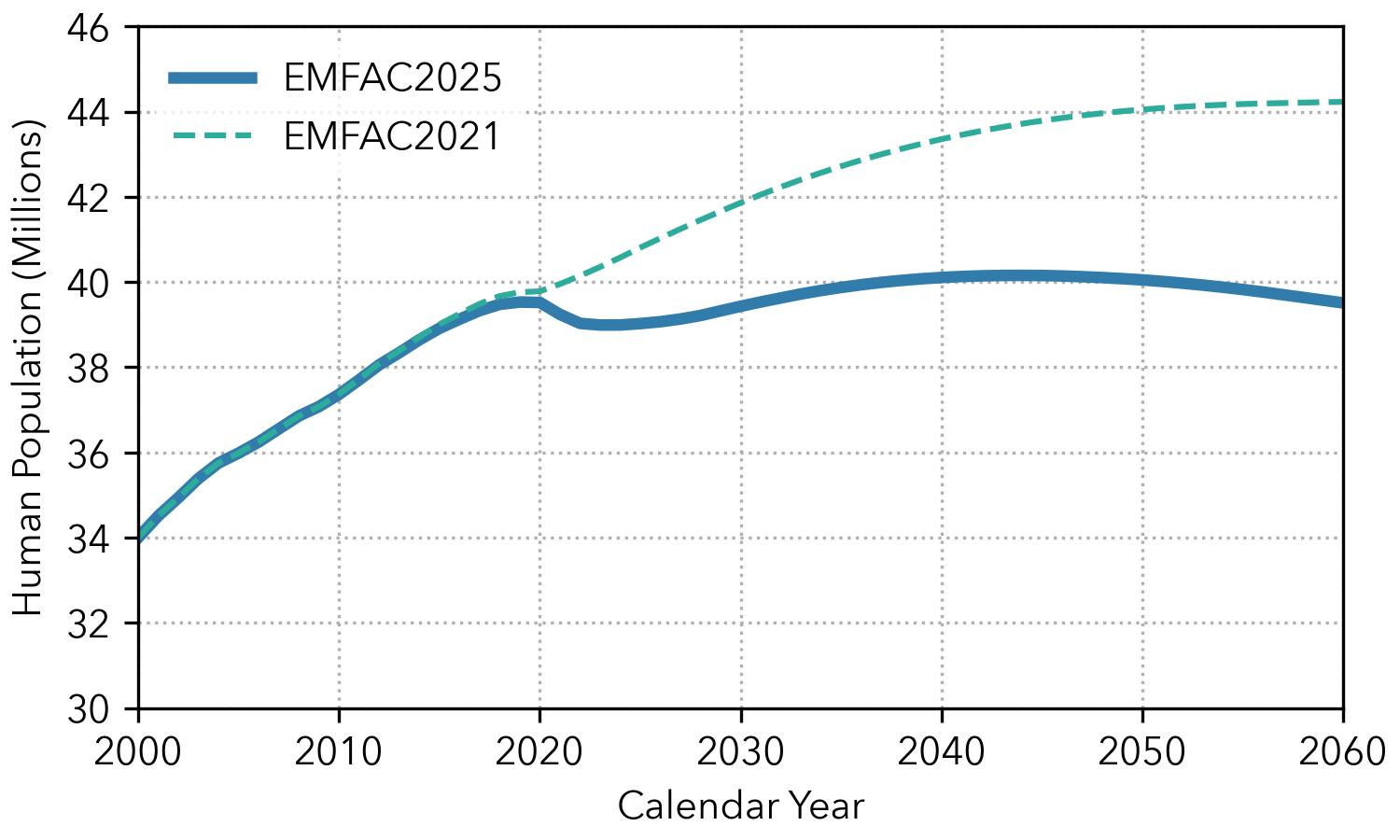
Figure 4.10: California’s Human Population Growth Forecast: EMFAC2025 vs. EMFAC2021#
To forecast VMT, CARB staff apply the human population growth rate relative to calendar year 2027 as shown in Equation (4.3):
where \(y\) is a given year between 2028–2050 and \(\text{Pop}\) is the human population. The resulting trend in future VMT is shown in Figure 4.11
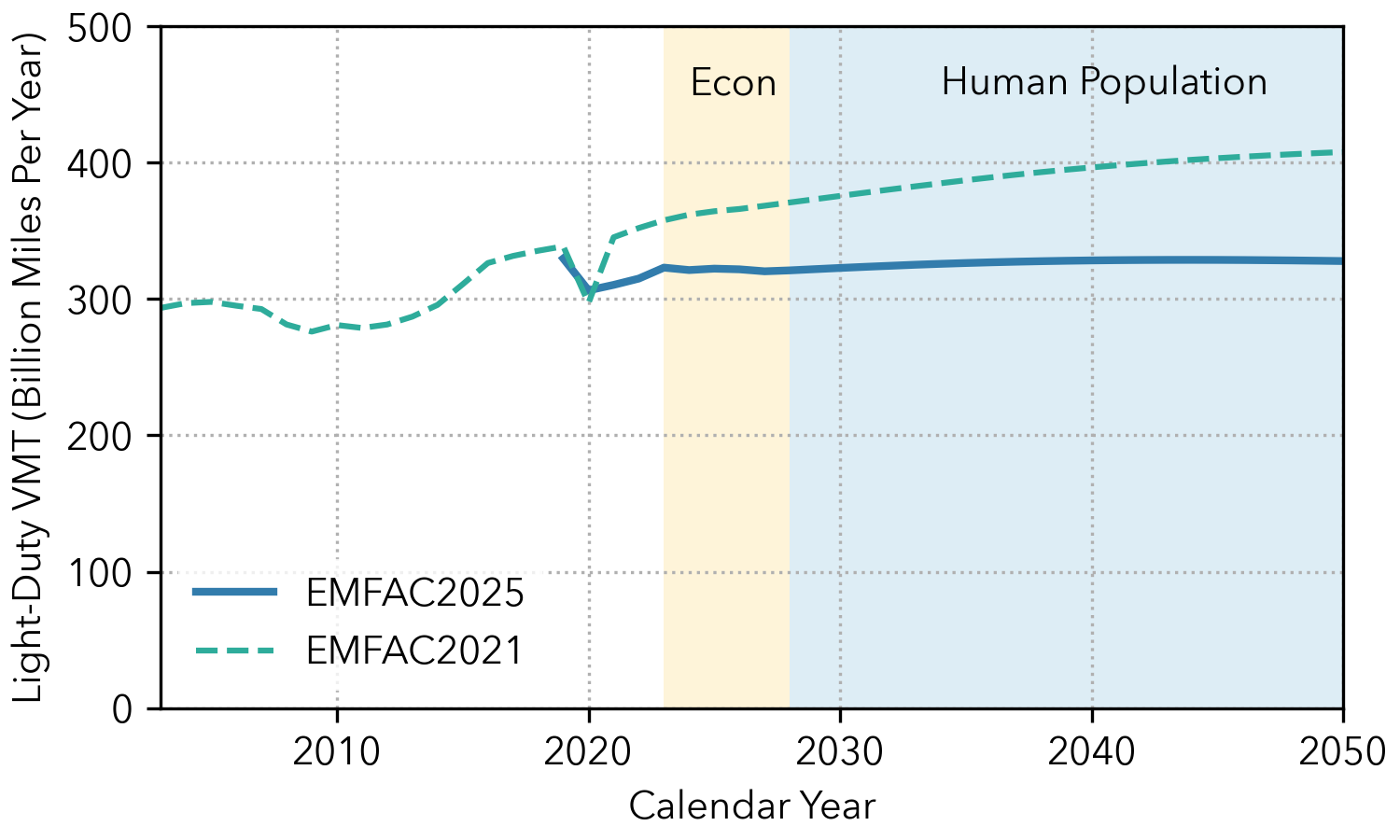
Figure 4.11: Forecasted Trends in Light-Duty Vehicle Miles Traveled, with Shaded Areas Indicating the Forecasting Methodology Used (Economic Multivariate Regression Model or Human Population Growth Rate).#
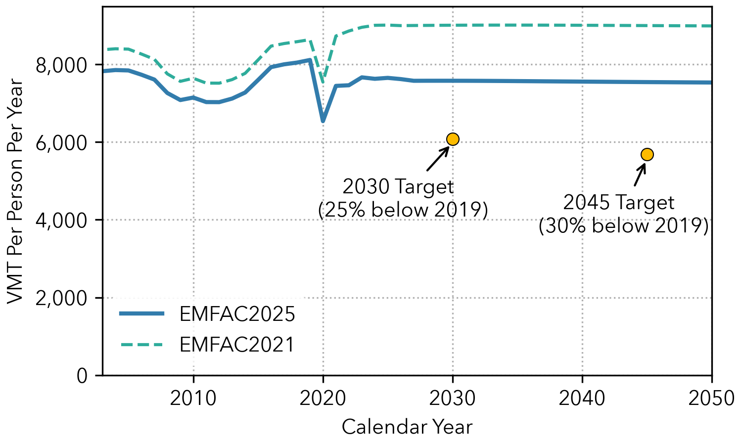
Figure 4.12: Forecasted Trends in Light-Duty Vehicle Miles Traveled Per Capita. Points indicate VMT per capita reduction targets (relative to calendar year 2019) set in the 2022 Scoping Plan.#
The EMFAC2025 forecast of VMT per capita (miles traveled per person per year) is shown in Figure 4.12. For pre-2020 historical years, EMFAC2025 estimates are consistently 6-7% lower than those in EMFAC2021. This reduction is primarily due to incorporation of high-speed driving, which decreased fuel efficiency. Since historical VMT is constrained by gasoline sales, the reduced fuel economy at higher speeds results in lower VMT estimates. After calendar year 2020, the gap in VMT per capita widens to 15-16%. The additional 8-9% difference is due to a slower post-pandemic VMT rebound than EMFAC2021 forecasted.
CARB’s 2022 Scoping Plan established targets to reduce VMT per capita by 25% by 2030 and 30% by 2045, relative to 2019 levels. Based on fuel sales, VMT per capita in 2024 is 6% below 2019, indicating modest progress towards the 2030 target.
4.4.2. Light-Duty New Vehicle Sales Forecast#
Forecasted light-duty vehicle populations are determined by estimating the number of vehicles retained from the prior calendar year and adding in the estimated new vehicle sales, where new vehicle sales are exclusively the sales of brand new automobiles and does not include used vehicle sales. Figure 4.13 illustrates this process for EMFAC2021, where a multivariable regression was used to estimate forecasted new vehicle sales.
In EMFAC2021, the forecasting equation for statewide new sales of light-duty vehicles, of all fuel types, was developed using a multivariable regression analysis based on historical socio-econometric time-series data. EMFAC2021 included a modeling approach where variables were chosen based on the socio-economic indicators that best described the historical trend in new vehicle sales per capita. The primary data sources used for this analysis included UCLA Anderson Forecast (UCLA), California Department of Finance (DOF), and Department of Motor Vehicles (DMV) registration data.
        flowchart LR
   A["<b>Multivariable Regression</b>"] --> B["<b>Forecasted<br> New  Vehicle Sales</b>"]
   B --> C["<b>Forecasted Population (Total Vehicles)</b>"]
   D["<b>Changes in<br> Historical DMV Registration</b>"] --> E["<b>Vehicle Retention Rates</b>"]
   E --> C
   classDef default stroke-width:3px,fill:#ffffff
   classDef carbnavy color:#1b577d,stroke:#1b577d
   classDef carbblue color:#327cac,stroke:#327cac
   classDef carbgreen color:#2fa596,stroke:#2fa596
   classDef carbyellow color:#fcbc00,stroke:#fcbc00
   class A,B carbblue
   class C carbnavy
   class D,E carbgreen
Figure 4.13: EMFAC2021 Light-Duty Vehicle Population Forecasting Methodology#
For EMFAC2025, a multivariable regression analysis to forecast new vehicle sales per capita was only used for the short-run forecasting (calendar year \(<\) 2025) using a similar methodology as described above for EMFAC2021. Economic data provided by UCLA Anderson was used for the short-run forecasting. The data used in the regression analysis included gas price, GDP, interest rate, housing starts, unemployment, and disposable income as predictor variables. Since it is impractical to look at all available combinations of the given parameters, a model was developed to create random n-variable models using a combination of the given parameters such as housing starts and unemployment rate. Each model generated was then filtered based on their \(R^{2}\), \(p\)-values, and the sensibility of the coefficients (e.g., negative correlation between unemployment rate and new vehicle sales). The models were created based on historical socio-econometric data obtained for calendar years 2003 through 2021; and projection or forecast for new vehicle sales was developed for calendar years 2023 through 2050. As shown in Equation (4.4), the selected model for forecasting light-duty new vehicle sales (NVS) per capita is a function of unemployment rate and housing starts.
The selected model has an adjusted \(R^{2}\) of 0.77, and \(p\)-values less than 0.05 for each predictor value, illustrating the significance of the selected parameters. A two-variable regression was chosen for its simplicity and no significant increases in adjusted \(R^{2}\) or reductions in \(p\)-value when using higher order regressions. Table 4.7 shows coefficient values and \(p\)-values for each coefficient used in the regression.
Variable |
Coefficient |
\(p\)-Value |
|---|---|---|
\(y\)-intercept |
\(3.56\times10^{-2}\) |
\(5.7\times10^{-6}\) |
Housing Starts |
\(1.03\times10^{-4}\) |
\(4.4\times10^{-4}\) |
Unemployment Rate |
\(1.06\times10^{-6}\) |
\(3.4\times10^{-2}\) |
For the long-run forecasting (calendar year \(\ge\) 2025), an equilibrium model, developed from a CARB contract with University of California San Diego (Jacobsen, 2023), was used to estimate new vehicle sales. This change in methodology is highlighted in Figure 4.14 with changes shown in the orange boxes. The multivariable regression is necessary in the short-run due to many ongoing market externalities (e.g., COVID-19 pandemic and chip shortages in 2020 and 2021) that are impacting the new vehicle sales market. Thus, the short-run multivariable regression is used as a “bridge” between historical new sales and the long-run equilibrium model.
        flowchart LR
   A["<b>Multivariable Regression</b>"] --> B["<b>Forecasted<br> New  Vehicle Sales</b>"]
   B --> C["<b>Forecasted Population (Total Vehicles)</b>"]
   D["<b>Changes in<br> Historical DMV Registration</b>"] --> E["<b>Vehicle Retention Rates</b>"]
   E --> C
   F["<b>Long-Run Forecast using Equilibrium Model</b>"] --> B
   classDef default stroke-width:3px,fill:#ffffff
   classDef carbnavy color:#1b577d,stroke:#1b577d
   classDef carbblue color:#327cac,stroke:#327cac
   classDef carbgreen color:#2fa596,stroke:#2fa596
   classDef carbyellow color:#fcbc00,stroke:#fcbc00
   class A,F carbyellow
   class B carbblue
   class C carbnavy
   class D,E carbgreen
Figure 4.14: EMFAC2025 Light-Duty Vehicle Population Forecasting Methodology#
The long-run equilibrium model is a dynamic equilibrium model that determines the point where supply and demand of vehicles are in balance. For example, if there is reduced travel demand forecasted in the future (e.g., lower population, better public transport forecasted, etc.), the equilibrium model will adjust the estimated sales of new vehicles, as well as the retention for older vehicles in the fleet. By using VMT forecasting as a proxy for travel demand, the equilibrium model is better equipped to capture changes in new vehicle sales based on projected travel demand and the price of vehicles rather than solely relying on historical new vehicle sales trends, as is true with the multivariable regression modeling. Please see (Jacobsen, 2023) for more details on the equilibrium model development.
Figure 4.15 shows the results for the new vehicle sales forecast for EMFAC2025 separated into short-run and long-run forecasts. Figure 4.15 also shows historical new vehicle sales and the forecasted new vehicle sales in EMFAC2021. Overall, results show that there is a decrease in forecasted new vehicle sales for EMFAC2025 compared to EMFAC2021. As discussed previously, for calendar year \(<\) 2025, this decrease is largely due to slower economic growth predicted from UCLA Anderson’s economic forecast. For calendar year \(\ge\) 2025, the long-run forecast shows stagnant growth in new vehicle sales, which can largely be attributed to little to no growth in VMT as discussed in Section 4.4.1. Since EMFAC2025 forecasts minimal VMT growth, there will likely not be a significant increase in demand for new vehicle sales.
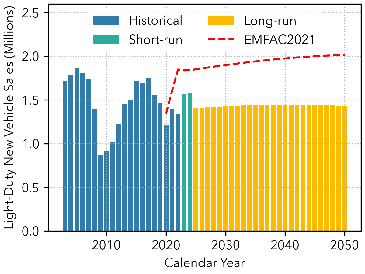
Figure 4.15: Forecasted New Vehicle Sales: EMFAC2025 vs. EMFAC2021#